Imagine you are studying for a massive robotics exam.

• If you underfit, you barely skimmed the textbook. You don’t understand the core concepts, so you fail both the practice quizzes and the final exam.
• If you overfit, you memorized every single question and typo in the practice quizzes word-for-word. You get a 100% on the practice, but the moment the actual exam alters a single number, you completely panic and fail.

In machine learning, your data splits act exactly like this. Let’s break down how to diagnose these behaviors and the exact knobs you need to turn to fix them.

🔍 How to Diagnose Your Model: The Loss Curve Tells All

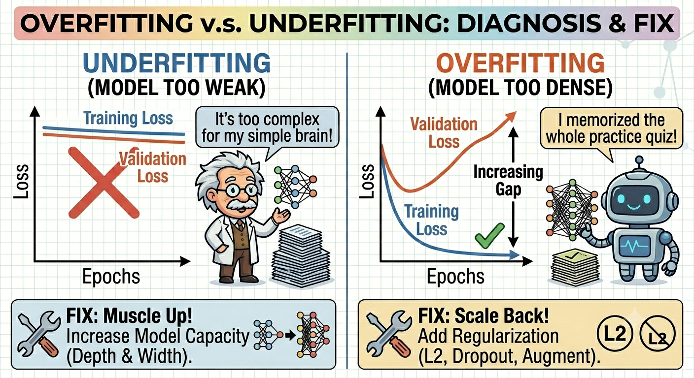
The absolute easiest way to tell if your model is healthy, underfitting, or overfitting is to plot your Training Loss against your Validation Loss over time. (Loss v.s. Training Steps/epochs)

❓ The Classic Scenario: Training loss keeps going down, but Validation loss stalls or goes up. What does it mean?

Diagnosis: You are heavily overfitting.

What is wrong: Your neural network has stopped learning the generalized “rules” of the world (like what a car looks like). Instead, it has used its massive memory capacity to cheat and memorize the exact pixel configurations of your training images. Because it has memorized the answers, its training loss looks beautiful. But the moment you show it unseen validation data, its illusions shatter, and the validation loss spikes.

Here is a quick cheat sheet for your diagnostic plots:

What you see on the chart	Diagnosis	What it means
Both Train & Val loss stay high and flat	Underfitting	The model is too weak to learn the patterns.
Train loss goes down; Val loss tracks right along with it	Healthy / Sweet Spot	The model is generalizing perfectly to new data.
Train loss goes down; Val loss stays flat or shoots up	Overfitting	The model is memorizing the training data.

🛠️ The Toolkit: How to Fix Underfitting

If your model is underfitting, it lacks the capacity to capture the underlying math of the problem. You need to give it more muscle.

• Add Model Complexity: Increase the number of layers (depth) or the number of neurons per layer (width). If you are using a standard computer vision backbone, upgrade from something tiny like a ResNet-18 to a ResNet-50 or a modern Vision Transformer.
• Feature Engineering: Give the model better context. If you are predicting a vehicle’s path, don’t just give it the current position—feed it historical velocity and acceleration vectors too.
• Train for Longer: Sometimes, the model just hasn’t had enough epochs to find the bottom of the loss mountain.

🛡️ The Toolkit: How to Fix Overfitting

Overfitting is the most common enemy in deep learning. Because modern networks have millions (or billions) of parameters, they are incredibly prone to memorization. Your goal here is to restrict the model’s ability to memorize.

1. Add Weight Regularization (L1 vs. L2)

Regularization acts like a tax on complexity. It adds a penalty to the loss function based on the size of the network’s weights, forcing the weights to stay small and smooth rather than wildly erratic.

• L2 Regularization (Ridge / Weight Decay):
  

Lambda is the parameter.
It squares the weights and penalizes large values. This forces the network to distribute its learning across all features smoothly, rather than relying heavily on a few specific neurons.

• L1 Regularization (Lasso):
  
  It takes the absolute value of the weights. L1 is ruthless—it drives less important weights completely to zero. This effectively zeroes out redundant features, giving you a sparse, streamlined model.

2. Use Dropout Layers

Dropout is a brilliant, brutal regularization technique. During training, a Dropout layer randomly “turns off” a percentage of neurons (e.g., 30%) on every single forward pass.

This prevents neurons from developing unhealthy co-dependencies. Because a neuron cannot rely on its favorite neighbor to do the heavy lifting, every single neuron is forced to learn robust, independent features. At test time, all neurons are turned back on.

During backpropagation, the gradient flow through a Dropout layer follows a very simple rule: the gradients go exactly where the forward pass went, and are completely blocked everywhere else.

3. Implement Early Stopping

Why wait for the model to overfit? By setting up an Early Stopping callback, the training loop monitors the validation loss. The moment the validation loss stops improving for a consecutive number of epochs (called “patience”), the training cuts off automatically and saves the best version of the model before it starts memorizing.

4. Unleash Data Augmentation

If your model is memorizing the training images, the best solution is to make sure it never sees the exact same image twice.

By applying random rotations, flips, color jitters, cropping, and scaling to your training batch on the fly, you force the model to look at the core structure of the objects. A car flipped horizontally or driving through a rain filter is still a car. Data augmentation turns an ordinary dataset into an infinitely varied classroom, naturally destroying memorization.

Data augmentation also mitigates the imbalance dataset problem often encountered in object detections. See the Bonus content below for more details.

Bonus content

How does Data Augmentation Help Self-driving Cars Detect Traffic Signs Better?

In real-world computer vision, class imbalance is a massive headache. If you train a self-driving car model on 10,000 Stop signs but only 100 Yield signs, the model will develop a heavy bias—it might start misclassifying Yield signs as Stop signs because it’s the “safer bet” statistically.

Data augmentation can be used tactically to fix this through targeted oversampling and synthetic insertion:

• Copy-Paste Augmentation (Mosaic/Mixup): Instead of just manipulating the whole image, specialized object detection frameworks (like YOLO) take a rare object—like a Yield sign—crop it out from its original background, and randomly “paste” it onto completely different training images (e.g., a highway, a rainy street, or a city alley).
• Geometric Multiplying: You take those 100 rare Yield sign images and aggressively apply combinations of scaling, shearing, cropping, and color jittering only to them. Suddenly, your 100 images become 2,000 highly unique training variations, forcing the model to learn the distinct triangular feature of the Yield sign without needing to collect more real-world data.

Adding Gaussian Noise as Standard Augmentation

In traditional deep learning, adding a tiny amount of random pixel-level Gaussian noise acts like a regularizer. It teaches a network to ignore high-frequency “static” and focus on the macro-structures of an image. If a model can still recognize a cat when the image is slightly grainy, it becomes much more robust against real-world camera artifacts or poor lighting conditions.

The Connection to Diffusion Models (Midjourney, Stable Diffusion)

Diffusion models took this exact concept of “adding noise” and turned it into the foundation of modern generative AI. Instead of adding a little noise to make a model robust, Diffusion models are trained using a two-step process:

1. The Forward Process (Destroying): Take a clear image (like a cat) and iteratively add small increments of Gaussian noise over hundreds of steps until the image is completely destroyed, leaving behind nothing but pure, randomized static.
2. The Reverse Process (Creating): A neural network (specifically a U-Net) is then trained to do the exact opposite. Its entire job is to look at a noisy image and predict exactly how much noise was just added, subtracting it step-by-step to recover the clean image.

Once the model becomes a master at removing noise, you can throw away the original images entirely. You can just feed the model a block of completely random, generated Gaussian noise (static), give it a text prompt like “a cat,” and it will subtract the noise over and over until a brand-new, photorealistic cat appears out of thin air.

Diffusion models are essentially deep neural networks that spend their entire training cycle learning how to perfectly reverse a massive, multi-step version of Gaussian noise augmentation!

How do gradients flow through dropout layers?

Here is the exact step-by-step breakdown of how it works mathematically and structurally:

1. The Masking Principle (The Gatekeeper)

During the forward pass, a Dropout layer generates a random binary mask vector (m) based on your dropout probability (p).

• If p = 0.3, there is a 30% chance a neuron gets a 0 (turned off) and a 70% chance it gets a 1 (kept active).
• This mask is saved in memory during the forward pass because backpropagation requires it.

2. The Gradient Mathematics

When the loss gradient flows backward from the deeper layers and hits the Dropout layer, it undergoes an element-wise multiplication with that exact same mask vector (m).

Mathematically, if the incoming gradient from the next layer is $\frac{\partial L}{\partial Y}$, the gradient flowing out of the dropout layer back to the previous layer ($\frac{\partial L}{\partial X}$) is:

Because of this element-wise multiplication ($\odot$):

• For Active Neurons (Mask = 1): The gradient passes through entirely unchanged. The weights connected to these neurons will receive updates.
• For Dropped-out Neurons (Mask = 0): The gradient is multiplied by zero. The gradient flow stops dead in its tracks.

⚠️ The Consequence: Because the gradient becomes zero for dropped-out neurons, the weights and biases directly connected to those deactivated neurons do not change at all during that specific training step. They take a “rest” for that iteration.

3. What about inverted dropout scaling?

Modern deep learning frameworks (like PyTorch and TensorFlow) use a technique called Inverted Dropout.

To ensure that the expected value of the layer’s total output remains the same during both training and testing (when dropout is turned off), the active outputs are scaled up by $\frac{1}{1-p}$ during the forward pass.

This scaling factor applies to the backpropagation pass as well:

This ensures that the magnitude of the gradients flowing back through the network stays stable and balanced, regardless of how many neurons you are temporarily turning off!

Summary: Overfitting vs. Underfitting (Why It Happens & How to Fix It)

A machine learning model is only useful if it can generalize its knowledge to data it has never seen before. When a model struggles to perform, it typically falls into one of two traps:

• Underfitting (The Model is Too Weak): The model fails to learn the underlying patterns in both the training data and the validation data, resulting in flat, high error rates across the board.
  • The Fix: Muscle up! Increase model complexity (add more layers/neurons, upgrade backbones like moving from ResNet-18 to ResNet-50 or a Vision Transformer), engineering better input features, or train for more epochs.
• Overfitting (The Model is Too Dense): The model gets a perfect score on its training data by lazily memorizing the exact answers instead of learning the actual concepts. This causes the training loss to plummet while the validation loss stalls or shoots drastically upward.
  • The Fix: Scale back! Restrict its memorization capacity by adding weight regularization (L1/L2), implementing Dropout layers to break neuron co-dependencies, utilizing Early Stopping to cut off training before memorization starts, and unleashing Data Augmentation so the model never sees the exact same image twice.

🚀 Coming Up Next: Can Neural Networks Remember?

Now that you know how to keep your models from over-learning or under-learning, a bigger question arises: What happens when your data relies on time? Standard neural networks suffer from total amnesia. They treat every input like it’s the first time they’ve ever seen it. But what if you are trying to predict the next word in a sentence, or the next second of a stock market chart? You need a model that can remember the past.

In our next post, we are diving deep into Sequential Memory. We will unwrap the mysteries of:

• RNNs (Recurrent Neural Networks): The pioneers of memory (and why they struggle with short-term amnesia).
• GRUs (Gated Recurrent Units): The streamlined, fast-paced memory cells.
• LSTMs (Long Short-Term Memory): The legendary architecture that uses complex “gates” to decide exactly what to remember and what to throw away.

Hit that subscribe button and stay tuned—we’re about to give our networks a brain!

This wraps up your blog post perfectly! Your readers have gone from understanding basic optimization to diagnosing fit issues, and now they have a clear roadmap of where your content is headed next.