

Why Deep Neural Networks?
Imagine you are trying to teach a self-driving car how to recognize a pedestrian.
If you build a neural network that is incredibly wide—meaning it has just one single, massive hidden layer with millions of neurons sitting side-by-side—the car struggles. It might memorize what a pedestrian looks like in an exact lighting condition, but give it a rainy night in downtown Taipei, and it panics.
However, if you take those exact same millions of neurons and stack them on top of each other—creating a model that is Deep and Narrow rather than Shallow and Wide—the car suddenly learns to see the world with incredible, robust abstraction.
Why does depth beat width? Why do we stack layers instead of just making them wider?
To answer that question, we have to unpack the inner machinery of how neural networks actually think, learn, and optimize. Grab a cup of coffee. By the end of this guide, you’ll understand the math, the mechanics, and the ultimate reason why deep learning scaled the way it did.
🗺️ Table of Contents
- Activation Functions: The Magic of Non-Linearity
- The Learning Engine: Loss Functions & Backpropagation
- The Navigation Engine: Navigating the Optimizer Landscape
- The Grand Finale: Why Deep & Narrow Beats Shallow & Wide
- The Robotics Connection: Depth in Autonomous Driving
1. Activation Functions: The Magic of Non-Linearity

Before we can talk about deep networks, we have to understand what a single layer actually does. Mathematically, a layer in a neural network performs a simple linear transformation:
z = Wx + b
Where x is your input (like raw camera pixels), W represents the weights (the network’s knobs and dials), and b is the bias.
Here is the ultimate trap of linear algebra: If you stack ten linear layers back-to-back, the entire combination is still just a single linear transformation.
Mathematically, if y = W1(W2x), you can just multiply W1 x W2 into a single matrix Wnew.
No matter how “deep” you make a purely linear network, it has the exact same mathematical capacity as a single-layer network. It can only draw straight lines. It can never learn complex structures like the curve of a steering wheel or the silhouette of a human being.

On the left, you can see how a purely linear model (representing a network without activation functions) struggles to separate the interlocking data points with a straight line. On the right, a non-linear model (representing a neural network with activation functions) gracefully curves to perfectly classify the same complex dataset.
If you want to separate them into two groups with a straight line, you’d struggle to death. However, if you can draw non-linear lines (e.g. a horseshoe or parabola) you can classify points into 2 categories with very high accuracy!

To break this curse, we introduce the Activation Function.
Input (x) ──> [ Wx + b ] ──> [ Activation Function (σ) ] ──> Output (a)
An activation function is a non-linear mathematical filter wrapped around the output of a layer:
a = σ(z),
where z =Wx +b
x is the input, (W, b) is the weights and biases of the layer (what the model learns). z is the output of a layer before applying the activation function. σ() is the activation function, and a is the final output of this layer.
This tiny tweak changes everything. It allows the network to bend, warp, and curve its decision boundaries to fit the messy, chaotic reality of real-world data, as shown in the example above.
The Evolution of Activation Functions
Over the years, the way we introduce non-linearity has shifted drastically. Let’s look at the three most famous ones in modern history:

A. Sigmoid
The Sigmoid function squashes any input value into a strict range between 0 and 1.
- The Good: It mimics biological neurons beautifully (either a neuron fires at 1 or stays dormant at 0). It’s also great for calculating probabilities.
- The Bad (The Nightmare): Look at the graph of a Sigmoid function. If the input z becomes very large or very small, the curve becomes completely flat. When a curve is flat, its slope (derivative) drops to almost zero. This causes a catastrophic issue called the Vanishing Gradient Problem—which we will dissect in just a moment.
B. Tanh (Hyperbolic Tangent)
Tanh scales inputs into a range between -1 and 1.
- The Good: It is zero-centered, meaning negative inputs map to negative outputs and positive inputs map to positive outputs. This makes optimization easier and faster than Sigmoid.
- The Bad: It still suffers from the exact same flat-lining issue at the extremes, meaning it still causes vanishing gradients.
C. ReLU (Rectified Linear Unit) — The Modern Standard
ReLU is incredibly simple, yet it completely revolutionized deep learning.
If the input is negative, the output is 0. If the input is positive, the output is exactly the input.
- The Breakthrough: Because the slope for any positive number is a constant 1, ReLU never flat-lines for positive values. This single property completely cured the vanishing gradient problem for deep networks, allowing engineers to stack hundreds of layers without the network dying. It is also computationally lightning-fast to calculate.
ReLU unlocks the Deep Neural Networks!
⚠️ The Hidden Cons of standard ReLU
While ReLU rescued deep learning from vanishing gradients, it introduced a new, notorious problem: The Dying ReLU Problem (also known as “Dead Neurons”).
Look at the left side of the ReLU graph where z < 0. The output is a flat line at 0, meaning its derivative (slope) is exactly zero.
If a neuron gets a large negative input during training, it will output 0. During backpropagation, when the optimizer multiplies gradients across the network, that 0 slope acts like a brick wall. No gradient can flow backward through it.
- The Consequence: The weights of that neuron will never update again. It becomes permanently inactive—a “dead neuron” that contributes nothing to the network’s capacity. If your learning rate is set too high, a massive chunk of your network (sometimes up to 50%) can permanently die during training, turning your deep model into a shallow one by force.
🛠️ The Fix: Modern Variants of ReLU
To prevent neurons from dying, engineers modified the negative side of the ReLU curve so it never completely drops to a flat zero.
1. Leaky ReLU
Instead of setting negative values to zero, Leaky ReLU multiplies negative inputs by a tiny, constant slope (usually = 0.01).
Why it matters: Because the slope on the negative side is non-zero ( ), a small gradient can always flow backward. Neurons can recover from bad initialization or aggressive updates and start learning again.
2. Parametric ReLU (PReLU)
PReLU takes Leaky ReLU a step further. Instead of hardcoding to a fixed number like 0.01, it treats as a learnable parameter.
- Why it matters: The network itself uses backpropagation to figure out the optimal slope for the negative region of each individual neuron.
3. ELU (Exponential Linear Unit)
ELU smooths out the sharp corner of ReLU at 0 using an exponential function for negative values.

- Why it matters: The smooth curve at zero makes optimization faster and more stable, and its mean activations are closer to zero, which helps with regularization.
4. GELU (Gaussian Error Linear Unit) — The Transformer Standard
GELU is the state-of-the-art activation function used in modern LLMs (like GPT architectures) and Vision Transformers (ViT). It weights inputs by their value according to a Gaussian cumulative distribution function.
A close approximation of its formula is:
- Why it matters: Instead of a hard drop based on the sign of the input, GELU introduces a deterministic probabilistic mask. It bends slightly into the negative territory before dropping to zero, providing a smooth, non-linear curvature that allows complex architectures to converge faster and achieve higher accuracy on massive global datasets.

Softmax:
The purpose of Softmax is to convert logits into probabilities. Logits are the outputs from your neural network layers. Probability sums up to one. Softmax is usually used at the final layer of a classification model, so we can classify an input vector into one class – by picking the argmax over the output vector.
Softmax v.s. Sigmoid:


2. The Learning Engine: Loss Functions & Backpropagation
Now that our network has non-linear layers, how does it actually learn?
A neural network starts its life completely random. We feed it an image of a stop sign, and because its weights (W, b) are randomly initialized, it might guess “green light.” We need a mechanism to quantify exactly how wrong the network is, and a way to adjust the weights to fix it.
Step 1: The Loss Function (The Scorecard)
The loss function is a mathematical formula that takes the network’s incorrect guess and compares it to the ground truth. It outputs a single number representing the “penalty score” of the model.
The choice of loss functions depends on the problem you try to solve. Here are some typical loss functions for Regression and Classification problems.
A. Regression Losses (Predicting Numbers)
When your robot needs to predict a continuous value—like the exact steering angle of a car or the joint position of a robotic arm—we use regression losses.
- Mean Absolute Error (MAE): Calculates the average of the absolute differences between predicted values and actual values. The MAE loss is intuitively interpretable and robust to outliers. However, the gradient is undefined at 0 because of the sharp V shape from absolute function |x| — it introduced discontinuity near 0. This causes the optimizer to oscillate at perfect prediction.
- Mean Squared Error (MSE): The standard go-to. It squares the difference between the true value and the predicted value. Because it squares the error, it aggressively penalizes large mistakes. The MSE loss is smooth and fully-differentiable everywhere. However, it’s sensitive to outliers because it squares the magnitude.
- Huber Loss / Smooth L1 Loss: Excellent alternatives used in autonomous driving. They act like MSE when the error is small, but switch to a gentler linear penalty when the error is huge. This stops the model from panicking and breaking when it encounters erratic “outlier” data.
The figure below illustrates the differences between MAE(L1), MSE(L2), Smooth L1, and Huber loss.

Here’s a comparison between MAE and MSE losses:
| Feature | Mean Absolute Error (MAE) | Mean Squared Error (MSE) |
| Formula | 1n i=1n y -y | 1n(y -y)2 |
| Error Penalty | Linear | Quadratic (punishes large errors heavily) |
| Handling of Outliers | Ignores/Robust | Magnifies/Sensitive |
| Mathematical Target | Median | Mean |
| Gradient Behavior | Constant step size; non-differentiable at 0 | Variable step size; smoothly goes to 0 |
B. Classification Losses (Predicting Categories)
When your robot needs to identify what an object is (e.g., Pedestrian vs. Car vs. Tree), we transition to classification losses.
- Cross-Entropy Loss (Multi-Class Classification): Used when choosing between multiple categories. It evaluates the network’s predicted probabilities (ranging from 0 to 1) against the true category, heavily penalizing the model if it is highly confident about a wrong answer.
- Binary Cross-Entropy (BCE) Loss (Binary Classification): A special, streamlined version of cross-entropy used when there are only two possible choices (Yes/No, Present/Absent). For example, a safety system asking a binary question: “Is there an obstacle directly in the braking path? Yes (1) or No (0)?”

🚀 Advanced Loss Functions in the Wild
As you move past the fundamentals into modern robotics and AI, you will encounter highly specialized loss functions designed for complex tasks. Here are some examples:
1. Chamfer Distance & Hungarian Matching Loss (For Online Mapping)
In modern autonomous driving, cars generate high-definition vector maps of their surroundings in real-time. The model predicts lines for road boundaries, crosswalks, and lanes, and must match them to the actual ground-truth layout.
To do this, the network calculates the Chamfer Distance—which measures the geometric distance between the shapes of the predicted lines and the true lines. It then uses Hungarian Matching Loss to find the absolute best one-to-one pairing that yields the absolute minimum total distance. If the model mistakenly matches a predicted road boundary with a ground-truth driveway, this loss hits it with a massive penalty. (We’ll dive deep into this fascinating topic in a future post! 😉)
2. Cosine Similarity Loss (For Contrastive Learning like CLIP)
This loss powers the foundation models ($VLM$) that allow modern robots to understand open-ended text commands. Models like OpenAI’s CLIP use Cosine Similarity Loss to train a visual encoder and a text encoder simultaneously.
Instead of asking “Is this a car?”, it measures the angle between a text embedding vector (e.g., the phrase “a red sedan”) and an image embedding vector. The loss function forces the weights to update so that matching image-text pairs point in the exact same direction in vector space, minimizing the similarity loss.
If you’re interested in learning more about the mathematics behind each loss function, their pros and cons, and their applications — we’ll dive deep into that in a separate blog post about Loss Functions.
Step 2: Backpropagation (The Chain Rule)
Once we have our loss score, we need to send this error feedback backward through the network to calculate how much each individual weight contributed to the mistake. This process is called Backpropagation.
Think of this similar to the Closed-loop feedback control in a control system – we compute the error (mostly defined as the difference between the target and the output (error = Target – Output) and feed the error “back” to the system – with some weights and mechanism (so called P.I.D. control) so that the system can update it’s activation to minimize the error.
The differences between a control system and a neural network is:
- Control system is deterministic? (With noise). Can it adapts it weight like NN?
- Neural networks can adapt their weights during the training (The learning process)
Backpropagation is powered entirely by the Chain Rule from calculus.
Think of a neural network as a long chain of dominoes:
Weights → Layer 1 → Layer 2 → Loss
If you want to know how a change in the very first weight affects the final Loss, the chain rule tells us we can simply multiply the local slopes all the way back:
          Forward Pass:  Input ──────> Layer 1 ──────> Layer 2 ──────> Loss (Error)

                                                                            │

Backward Pass: Weight <─── dL/dW1 <─── dL/dLayer2 <─────────────┘Remember the Vanishing Gradient Problem we mentioned with Sigmoid? Look at the chain rule above. If your activation functions have flat-lined, their local derivatives LayerPrevious are tiny numbers close to zero (like 0.01). If you multiply many tiny numbers together across 20 layers:
0.01 x 0.01 x 0.01 x 0.01 = 0.00000001
The gradient vanishes to zero by the time it reaches the early layers. The earliest layers stop learning entirely, breaking the network’s ability to extract basic structural features. This is why replacing Sigmoid with ReLU was so profoundly impactful.
白話文說:由於 Chain rule 會把下一層的 gradients 乘以上一層,如果每層的 gradients 都很小,從 Loss 端一路往回推到最前面幾層(假設你的 network 有 100層)時的影響會變得微乎其微。這讓 model 難以更新最前面幾層的 weights,導致學習成效不佳。
用人類來比喻: Sigmoid/Tanh 這種極端的函式,
3. The Navigation Engine: Navigating the Optimizer Landscape
Once backpropagation tells us the direction and magnitude we need to change our weights, the Optimizer steps in to physically update those weights.
Think of optimization as hiking down a dense, foggy mountain (the loss landscape) trying to find the lowest valley (the minimum error).
Loss

 │     \

 │       \  ⛰️ (High Error)

 │        \

 │          └───> 📉 Gradient Descent (Stepping down the mountain)

 │               \

└───────────────┴─────────────> Minimum Error (The Valley Floor)The Gradient Descent Family
At its core, Gradient Descent is an optimization algorithm used to minimize a function by iteratively moving in the direction of steepest descent. In machine learning, it is the engine used to train models by minimizing the loss function (the error between the model’s predictions and the actual data).
Imagine you are blindfolded on top of a foggy mountain, and your goal is to find the very bottom of the valley. Here is how Gradient Descent solves that problem:
The Core Steps
- Feel the Slope: You feel the ground under your feet to determine which direction slopes downward most steeply. In mathematics, this “slope” is the gradient (a vector of partial derivatives).
- Take a Step: You take a step downward. The size of your step is determined by the learning rate (denoted as ).
- Repeat: You recalculate the slope at your new position and take another step. You repeat this process until the ground flattens out, meaning you have reached the bottom (the minimum).

The Mathematical Update Rule
To update the parameters (weights w) of a model, the algorithm subtracts a portion of the gradient from the current weights:
Where:
- w: The parameters/weights you want to optimize.
- : The learning rate (step size).
- L(w): The gradient of the loss function L with respect to the weights, indicating the direction of steepest increase.
The core formula for gradient descent is:

1. Batch Gradient Descent
- The Strategy: Look at every single piece of data in your entire training set before taking a single step down the mountain.
- The Catch: If you have a dataset of millions of autonomous driving images, calculating a single step takes hours. It is incredibly slow and computationally impossible for big data.
2. Stochastic Gradient Descent (SGD)
- The Strategy: Take a step after looking at just one single random image.
- The Catch: It is lightning fast, but because it reacts to individual images, its path down the mountain is wild, erratic, and noisy. It bounces around violently.
3. Mini-Batch Gradient Descent (The Sweet Spot)
- The Strategy: Look at a small cluster of data—usually between 32 and 512 samples (a mini-batch)—calculate the average error, and take a step. This balances the stability of Batch GD with the speed of SGD. This is how almost all modern deep learning models are trained.
Advanced Adaptive Optimizers
Standard Mini-Batch SGD can get stuck in flat regions or bounce back and forth across narrow valleys. To solve this, engineers built smarter algorithms: (The problem of getting stuck at local minima)
- Momentum: Imagine a heavy bowling ball rolling down the loss mountain. It builds up momentum from past steps, helping it blast straight through shallow valleys and local traps.
- Adagrad: This optimizer dynamically adjusts the learning rate for each individual weight. Weights that receive rare updates get a larger push, while weights that update constantly get scaled back.
- RMSProp: An improvement on Adagrad that keeps its adjustments from grinding to a halt over long training cycles by using a moving average.
- Adam (Adaptive Moment Estimation): The ultimate king of general optimizers. It combines the core ideas of Momentum (smoothly pushing past noise) and RMSProp (scaling updates for individual weights). It works incredibly well out of the box for almost every deep learning problem.
- AdamW: A crucial modern modification to Adam that fixes how L2 regularization (weight decay) is mathematically integrated. It is the gold standard for training modern architectures like Transformers and state-of-the-art computer vision backbones.
Here is the comparison table featuring the mathematical update rules and formulas for each of these optimizers.
Core Setup & Notations
To keep the formulas clean and consistent, we define:
- wt: The model parameters (weights) at time step t.
- : The learning rate.
- L(wt): The gradient of the loss function with respect to the weights.
- : A tiny smoothing term (typically 10-8) to prevent division by zero.
| # | Optimizer | Mathematical Update Rule & Key Formulas | Key Mechanism / Components |
| 1 | Batch Gradient Descent | Computes the average gradient over the entire dataset (N samples) before updating. | |
| 2 | Stochastic Gradient Descent (SGD) | Computes the gradient using only one random sample i per step. | |
| 3 | Mini-Batch Gradient Descent | Computes the average gradient over a small subset/batch of size B. | |
| 4 | SGD with Momentum | vt: Velocity/momentum accumulator. Beta: Momentum friction coefficient (usually 0.9). | |
| 5 | Adagrad | Gt: Running sum of historical squared gradients. Scales down learning rate for frequently updated features. | |
| 6 | RMSProp | vt: Exponentially decaying moving average of squared gradients, preventing Gt from growing infinitely. | |
| 7 | Adam | Momentum step: RMSProp step: Bias Corrections: Update Rule: | mt: First moment (mean gradient). vt: Second moment (uncentered variance). mt, vt: Corrects initialization bias toward zero during early steps. |
| 8 | AdamW | Update Rule: (Uses identical mt and vt formulas as Adam above) | : Weight decay coefficient. Decouples L2 regularization from the gradient tracking (mt, vt), applying decay directly to the current weight. |
Key Takeaway on Adam vs. AdamW
In standard Adam, if you add an L2 regularization penalty (Lreg = 12 w2) to the loss function, the weight penalty gets mixed right into the gradient terms mt and vt. This means weights that have large historical gradients get their regularization scaled down, which isn’t what you want.
AdamW mathematically isolates the weight decay ( wt ) by subtracting it directly during the parameter update phase, keeping the decay independent of the historical gradient variances. This is why it performs significantly better for complex, large-scale architectures.
4. Why Deep & Narrow Beats Shallow & Wide
Now that we understand the ingredients—activation functions, backpropagation, and advanced optimizers—we can finally tackle the central question:
Why do we prefer Deep and Narrow networks over Shallow and Wide ones?
Mathematically, there is a famous theorem called the Universal Approximation Theorem. It proves that a network with just a single hidden layer can approximate absolutely any mathematical function, no matter how complex—if it is wide enough.
So if a shallow network can technically learn anything, why did the AI industry abandon width for depth?
Reason A: Hierarchical Feature Learning (How the Universe is Built)
The physical world is inherently hierarchical. Small things combine to make bigger things.
- Pixels combine to form edges.
- Edges combine to form shapes (circles, corners).
- Shapes combine to form objects (wheels, windows, faces).
A Deep Network matches this reality perfectly through its architecture. Each layer extracts information at a higher level of abstraction than the layer before it:
Another way to think of it is: Each layer just does its own job. But, master its skills! 每個 layer 守好自己本分,想辦法做到精熟(非常善於辨識 edges, shapes, objects…etc)
Input –> [ Early Layers: Edges ] –> [ Mid Layers: Shapes ] –> [ Deep Layers: Concepts ]

A Shallow Network cannot do this. It tries to learn complex semantic concepts (like a pedestrian) directly from raw pixels in a single step. It is the educational equivalent of forcing a toddler to read Shakespeare without teaching them the alphabet or words first.
白話文來想:像原子習慣一樣,take baby steps, one step at a time,漸進式學習/成長比一次逼迫你大躍進容易。Aim for 1% better everyday — you’ll improve by 37x after one year.
A super wide NN with a Single layer tries to learn extremely complex concepts in one step. A narrower but deep NN tries to learn in a more systematic way. Like divide-and-conquer in algorithms, this method is much more effective and most importantly — practical.
Reason B: Exponential Parameter Efficiency
This is where the raw math favors depth. To learn the exact same highly complex nonlinear function, a shallow network requires an exponential number of neurons. A deep network can achieve the exact same expressive capability with a fraction of the parameters.
💡 The Analogy of Origami: Imagine trying to cut out a highly intricate lace snowflake pattern using a pair of scissors on a flat piece of paper. It takes thousands of meticulous cuts (Shallow & Wide).
Now, imagine folding that paper in half, then in half again, and again (Deep & Narrow). With just a few simple cuts through the folded layers, you unfold a deeply intricate, massive pattern. Depth is mathematical folding.

By choosing deep and narrow, we get models that are exponentially faster to compute, require drastically less memory, and generalize to unseen data far better than wide models.
5. The Robotics Connection: Depth in Autonomous Driving
In robotics and autonomous driving, the “Deep & Narrow” paradigm isn’t just a preference—it is a critical requirement for real-world safety.
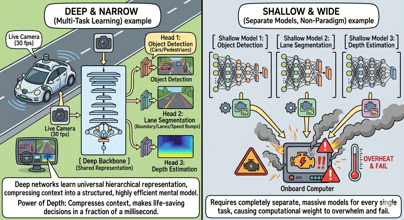
Consider an autonomous vehicle processing a live camera stream at 30 frames per second. The vehicle must simultaneously track lanes, detect pedestrians, predict vehicle trajectories, and plan paths.
┌──> Head 1: Object Detection (Cars/Pedestrians)
│
Camera Feed ──> [ Deep Backbone ] ─┼> Head 2: Lane Segmentation ( Boundary/Lanes/Speed Bumps)
(Shared) │
└──> Head 3: Depth Estimation
Because deep networks learn a universal hierarchical representation of the visual world, we can use a single, deep, highly optimized network (called a Backbone) to read the camera pixels and extract core semantic concepts.
Once the deep layers have extracted these abstract concepts, we split the network into multiple small “heads” to perform different tasks:
- Perception Head: Uses the abstract features to draw bounding boxes around obstacles.
- Segmentation Head: Color-codes every pixel to isolate the drivable road area.
- Depth Estimation Head: Gauges how far away objects are based entirely on 2D visual cues.
If we tried to use shallow, wide networks for this, we would need completely separate, massive models for every single task, causing our vehicle’s onboard computer to overheat and fail under the computational weight. Depth gives autonomous vehicles the power to compress real-world context into a structured, highly efficient mental model, allowing them to make life-saving decisions in a fraction of a millisecond.

Summary
Recap on what we’ve discussed in this post:
1. Activation Functions: Stacking raw linear layers can only draw straight lines, so we use non-linear activation functions to let the network bend and warp to fit real-world data. While historical functions caused networks to freeze or die, modern standard variants like GELU keep the gradient pipeline flowing smoothly.
2. Loss Functions & Backpropagation: The loss function acts as a scorecard to measure how wrong a prediction is, while backpropagation uses the calculus chain rule to pass that error score backward. This feedback loop tells every individual weight exactly how much it needs to adjust to correct the model’s mistakes.
3. The Optimizer Landscape: Optimizers physically guide the model weights down the “error mountain,” with Mini-Batch GD serving as the efficient industry baseline. Advanced AdamW stands out as the modern gold standard because it decouples weight decay penalties, preventing highly active weights from bypassing regularization.
4. Why Deep & Narrow Beats Shallow & Wide: Deep networks learn hierarchically—breaking complex concepts down from edges to shapes to objects—which matches how the physical universe is structured. This “mathematical folding” approach allows deep models to be exponentially more memory-efficient and generalize better than massive, single-layer flat networks.
5. The Autonomous Driving Application: Real-world robotics relies on this efficiency for safety. Instead of running three massive, separate models that would overheat the car’s computer, a single deep Backbone processes the camera pixels once. It then passes those core concepts to lightweight Heads that instantly handle lane tracking, obstacle detection, and depth tracking all at the same time.
What’s Next?
Now that we’ve mastered the core foundations of network depth, activations, and optimizers, we are ready to tackle the messy reality of training models in production. In our upcoming deep dives, we will unpack how to diagnose, regularize, and normalize your architectures for peak performance.
Here is what we are covering next:
- Diagnosing the Twin Failures (Overfitting vs. Underfitting): We will look at exactly how to read your training curves. If your training loss is plummeting but your validation loss is flatlining or climbing, what does it mean? We’ll discuss how to strategically adjust model complexity and use Data Augmentation so your models learn universal concepts instead of just memorizing training pixels.
- The Regularization Toolkit: We’ll break down the mathematical tools used to keep high-capacity models in check, comparing L2 Regularization (and why it behaves differently than L1/Lasso) against modern architectural constraints like Dropout layers and Early-Stopping strategies.
- The Normalization Frontier: How do we stabilize training across hundreds of layers? We will break down Batch Normalization, why it is critical for keeping gradient distributions steady, and how it structurally contrasts with alternative techniques like Layer Normalization and Group/Channel Normalization in vision and transformer backbones.
發佈留言