

Have you ever wondered how a self-driving car actually “sees” a pedestrian?
To our human brains, spotting a person crossing the street feels instantaneous. But to a computer, an image isn’t a picture—it’s just a massive grid of numbers representing pixel colors.
When the modern era of Deep Learning began, engineers tried to feed these grids of numbers directly into standard neural networks called Multi-Layer Perceptrons (MLPs). It seemed logical: connect every single pixel to the network and let it figure it out.
Instead, the networks choked. They ran out of memory, forgot where things were, and failed at the simplest tasks.
To build vision systems capable of safely navigating a 4,000-pound autonomous vehicle through city streets, AI had to completely change its approach. This is the story of how we moved from the brute-force memorization of MLPs to the elegant, biologically inspired architecture of Convolutional Neural Networks (CNNs).
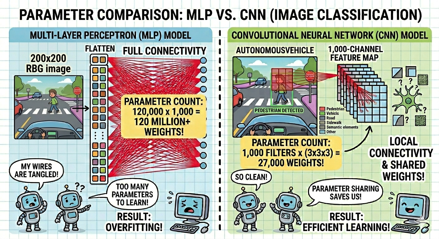
1. The Core Problem: The Multi-Layer Perceptron (MLP)
An MLP is a fully connected network. This means every single pixel of an input image must connect to every single neuron in the next layer.
At first glance, this sounds powerful. But let’s look at the math.
Imagine a relatively small color camera image on a robot: 200 x 200 pixels. Because it’s a color image, it has 3 channels (Red, Green, Blue).
Input Dimensions = 200 x 200 x 3 = 120,000 numbers
If your very first hidden layer is modest—say, just 1,000 neurons—the network has to calculate a weight matrix for every single connection:
120,000 x 1,000 = 120,000,000 parameters

120 million weights for just one single layer! If you try to scale this to a standard high-definition vehicle camera, the parameter count explodes into billions. This creates three critical failures:
- Overfitting (The Memorization Trap): With too many parameters, the model easily memorizes the exact training images instead of learning general patterns. It learns what a specific cat looks like, not what cats look like.
- Loss of Spatial Topology: MLPs force you to “flatten” a 2D image into a 1D long line of numbers. This completely destroys spatial relationships. The network treats pixels that are right next to each other exactly the same as pixels on opposite corners of the image.
- Lack of Translation Invariance: If an MLP learns to recognize a stop sign in the top-left corner of its camera view, it cannot automatically recognize that same stop sign if it shifts to the bottom-right corner. It has to relearn the concept of a stop sign all over again for that new location.
2. The Breakthrough: Stealing from Nature
To solve this scaling disaster, computer scientists stopped looking at pure computer code and started looking at biology.
In 1959, two neuroscientists named David Hubel and Torsten Wiesel ran a series of famous experiments on the visual cortex of mammals. They discovered two incredible things about how brains process sight:
- Local Receptive Fields: Individual neurons in your eyes and brain don’t look at the whole world at once. Each neuron only responds to stimuli in a highly restricted, local region of space.
- Simple vs. Complex Cells: Some cells act as “edge detectors”—they only fire when they see a sharp vertical or horizontal line in their tiny window. Other, more complex cells combine those inputs to detect motion or complex structures, regardless of their exact position.
In 1998, AI pioneer Yann LeCun formalized these biological shortcuts into modern deep learning with an architecture called LeNet-5. This was the birth of the Convolutional Neural Network (CNN).
3. The Solution: How CNNs Work
CNNs introduced two foundational ideas that drastically cut down parameters while making the network incredibly smart about space: Locality and Shared Weights.
A. Locality (Spatial Locality)
Instead of connecting a neuron to every pixel across the entire image, a CNN neuron only connects to a tiny, local region (like a 3×3 or 5×5 window).
The core assumption here is that nearby pixels are highly correlated. To find a pedestrian’s eye, you only need to look at the pixels immediately surrounding it—you don’t need to look at the asphalt under the car at the same time.
B. Shared Weights (Parameter Sharing)
In an MLP, every single connection has its own unique weight. In a CNN, a small block of weights—called a kernel or a filter—slides (convolves) across the entire image.
If a 3×3 filter is designed to detect a vertical edge, it uses the exact same 9 weights whether it is looking at the sky, a lane line, or a sidewalk.
This drastically reduces parameters. Because the same filter is reused everywhere, it gives the network Translation Invariance. If a feature is useful in one part of the image, it is useful everywhere.

4. The Secret Weapon: Pooling Layers
Once the convolutional layers extract these features, CNNs use another tool called a Pooling Layer (most commonly Max Pooling) to downsample the image.
Imagine a convolutional layer detects a sharp feature—like the corner of a truck—and outputs a high intensity value of 9. If the truck moves slightly due to a bump in the road, that 9 shifts by one pixel.
A Max Pooling layer looks at a small window (usually 2×2 pixels) and says: “I only care about the maximum value in this zone.”
Look at how the math handles this shift:
Plaintext
Original Feature Map:
[ (9  8)  4  4 ]  --> Max Pool Window (Top-Left): Max(9, 8, 5, 1) = 9
[ (5  1)  3  6 ]

Shifted Map (Truck moves 1 pixel to the right):
[ (0  9)  8  4 ]  --> Max Pool Window (Top-Left): Max(0, 9, 5, 1) = 9
[ (5  1)  3  6 ]
Even though the feature physically moved, the output of the pooling layer remains exactly 9.
This grants the network Local Translation Invariance. To the deeper layers of a self-driving car’s brain, the exact pixel coordinate doesn’t matter anymore. The network just registers a high-level concept: “The feature ‘truck corner’ is present in this general area.”
⚠️ Important Distinction: Locality vs. Invariance
As you build neural networks, don’t confuse these two terms:
- Locality is a boundary constraint enforced by Convolution: “I will only look at pixels that are close together.”
- Invariance is a flexibility property created by Pooling: “If a pattern moves slightly within those boundaries, I will still recognize it.”
🎬 Summary: The Ultimate Paradigm Shift
By swapping global, brute-force connectivity for elegant spatial shortcuts, CNNs allowed computers to transition from memorizing raw pixels to structurally understanding the visual world.
| Feature | Multi-Layer Perceptron (MLP) | Convolutional Neural Network (CNN) |
| Input Format | Flattened 1D vector | Native 2D or 3D tensor (Width x Height x Channels) |
| Connectivity | Fully Connected (Global) | Locally Connected (Local regions) |
| Weights | Unique weight for every single connection | Shared weights across the entire image |
| Parameter Efficiency | Extremely low (Scales poorly) | Extremely high (Independent of image size) |
| Spatial Awareness | None (Treats pixels independently) | Preserves spatial structures and pixel relationships |
Because of this architectural leap, modern autonomous vehicles can process high-resolution camera feeds in milliseconds, paving the way for safe, real-time perception.

What’s next?
In our next post, we’ll move from standard CNNs into the architecture that powers modern computer vision backbones, exploring how deep neural networks scale up to handle complex scenes. Stay tuned!